class FeatureGenerator:# these are hardcoded (after previously looking at the skewed columns) to exclude columns you don't want to log-scale, e.g. segment cols, target. # lists in order of client, forecast, historical, electricity, gas dfs skewed_cols = [ ['eic_count', 'installed_capacity'], ['direct_solar_radiation', 'surface_solar_radiation_downwards', 'snowfall', 'total_precipitation'], ['rain', 'snowfall', 'windspeed_10m', 'shortwave_radiation', 'direct_solar_radiation', 'diffuse_radiation'], ['euros_per_mwh'], ['lowest_price_per_mwh', 'highest_price_per_mwh'] ]def__init__(self, data_storage:Storage):self.data_storage = data_storagedef log_scale_df(self, df:pd.DataFrame, skewed_cols:list):# add log scaled columnsfor col in skewed_cols: df[f"log_{col}"] = np.log(df[col]+1)# drop the original skewed columns df.drop(columns=skewed_cols, inplace=True)return dfdef log_scale(self, dfs:list, skewed_cols:list):# not logging targetfor i, (df, cols) inenumerate(zip(dfs, skewed_cols)):self.log_scale_df(df, cols)def add_client_features(self, features_df:pd.DataFrame, client_df:pd.DataFrame): # to align w/ forecast horizon, shift dates 2 days forward (equivalent to 48h lag) client_df.loc[:, 'date'] = client_df.loc[:, 'date'] + pd.Timedelta(days=2)# create date column in train_df to join on (will drop after) features_df['date'] = pd.to_datetime(features_df['datetime'].dt.date)# join features_df = features_df.merge(client_df, how='left', on=['county', 'is_business', 'product_type', 'date']) features_df.drop(columns=['date'], axis=1, inplace=True)# indicate lag features_df.rename(columns={'log_eic_count': 'log_eic_count_48h', 'log_installed_capacity': 'log_installed_capacity_48h'}, inplace=True)return features_dfdef _reduce_float64(self, df:pd.DataFrame): float64_cols = df.select_dtypes(include=['float64']).columns.tolist()for col in float64_cols: df[col] = df[col].astype('float32')return dfdef _add_lagged_targets(self, df:pd.DataFrame, target_cols:list, lags:list):""" df (DataFrame): revealed targets target_cols (list): relevant columns to generate the lags and left join lags (list): hours to lag """ next_df = df.loc[:, target_cols]for lag in lags: next_df.loc[:, 'datetime'] = next_df.loc[:, 'datetime'] + pd.Timedelta(hours=lag) df = df.merge(next_df, how='left', on=['county', 'is_business', 'product_type', 'is_consumption', 'datetime'], suffixes=("", f"_{lag}h"))# subtract the lag added (reset the datetime back to original) next_df.loc[:, 'datetime'] = next_df.loc[:, 'datetime'] - pd.Timedelta(hours=lag)del next_df gc.collect()return dfdef _add_lagged_target_stats(self, df:pd.DataFrame, cols:list, agg_col:str, stat:str, lags:list):""" df (DataFrame): summary stats {mean,std} generated from revealed targets wrt {is_consumption,county,product_type,is_business} cols (list): relevant columns to generate the lags and left join agg_col (str): columns over which the summary stat was generated via a groupby stat (str): indicate the summary stat to lag lags (list): hours to lag """ next_df = df.loc[:, cols]for lag in lags: next_df.loc[:, 'datetime'] = next_df.loc[:, 'datetime'] + pd.Timedelta(hours=lag) df = df.merge(next_df, how='left', on=cols[:-1], suffixes=("", f"_{agg_col}_{stat}_{lag}h"))# subtract the lag added (reset the datetime back to original) next_df.loc[:, 'datetime'] = next_df.loc[:, 'datetime'] - pd.Timedelta(hours=lag)del next_df gc.collect()return dfdef _add_target_features(self, features_df:pd.DataFrame):## prelims############################################################### calculate aggregated stats #### mean production/consumption over all segments (county-is_business-product_type) for each datetime cons_cols = ['datetime', 'is_consumption', 'target'] is_cons_mean = features_df.drop(columns=['row_id']).groupby(['datetime', 'is_consumption'], as_index=False).mean()[cons_cols] is_cons_std = features_df.drop(columns=['row_id']).groupby(['datetime', 'is_consumption'], as_index=False).std()[cons_cols]## following capture more rows per aggregated stat than grouping over each segment ### mean production/consumption over all segments for each county for each datetime county_cols = ['datetime', 'county', 'is_consumption', 'target'] county_mean = features_df.drop(columns=['row_id']).groupby(['datetime', 'county', 'is_consumption'], as_index=False).mean()[county_cols] county_std = features_df.drop(columns=['row_id']).groupby(['datetime', 'county', 'is_consumption'], as_index=False).std()[county_cols]# mean production/consumption over all businesses/on-businesses for each datetime business_cols = ['datetime', 'is_business', 'is_consumption','target'] is_business_mean = features_df.drop(columns=['row_id']).groupby(['datetime', 'is_business', 'is_consumption'], as_index=False).mean()[business_cols] is_business_std = features_df.drop(columns=['row_id']).groupby(['datetime', 'is_business', 'is_consumption'], as_index=False).std()[business_cols]# mean production/consumption over all product types for each datetime product_cols = ['datetime', 'product_type', 'is_consumption','target'] product_type_mean = features_df.drop(columns=['row_id']).groupby(['datetime', 'product_type', 'is_consumption'], as_index=False).mean()[product_cols] product_type_std = features_df.drop(columns=['row_id']).groupby(['datetime', 'product_type', 'is_consumption'], as_index=False).std()[product_cols]### add lags for 2, 3, 4, 5, 6, 7, and 14 days #### cannot add 24h lag b/c minimum lag available (revealed targets) is 48h; 24h lag would introduce leakage. is_cons_mean =self._add_lagged_target_stats(is_cons_mean, cons_cols, "is_cons", "mean", [2*24, 3*24, 4*24, 5*24, 6*24, 7*24, 14*24]) is_cons_std =self._add_lagged_target_stats(is_cons_std, cons_cols, "is_cons", "std", [2*24, 3*24, 4*24, 5*24, 6*24, 7*24, 14*24]) county_mean =self._add_lagged_target_stats(county_mean, county_cols, "county", "mean", [2*24, 3*24, 4*24, 5*24, 6*24, 7*24, 14*24]) county_std =self._add_lagged_target_stats(county_std, county_cols, "county", "std", [2*24, 3*24, 4*24, 5*24, 6*24, 7*24, 14*24]) is_business_mean =self._add_lagged_target_stats(is_business_mean, business_cols, "is_business", "mean", [2*24, 3*24, 4*24, 5*24, 6*24, 7*24, 14*24]) is_business_std =self._add_lagged_target_stats(is_business_std, business_cols, "is_business", "std", [2*24, 3*24, 4*24, 5*24, 6*24, 7*24, 14*24]) product_type_mean =self._add_lagged_target_stats(product_type_mean, product_cols, "product_type", "mean", [2*24, 3*24, 4*24, 5*24, 6*24, 7*24, 14*24]) product_type_std =self._add_lagged_target_stats(product_type_std, product_cols, "product_type", "std", [2*24, 3*24, 4*24, 5*24, 6*24, 7*24, 14*24]) dfs = [is_cons_mean, is_cons_std, county_mean, county_std, is_business_mean, is_business_std, product_type_mean, product_type_std]for df in dfs: df =self._reduce_float64(df)# drop target column from the stats b/c mean of same day target introduces leakage df.drop(columns=['target'], axis=1, inplace=True)############################################################## add revealed targets; lagged 2, 3, 4, 5, 6, 7, and 14 days ## target_cols = ['target', 'county', 'is_business', 'product_type', 'is_consumption', 'datetime'] features_df =self._add_lagged_targets(features_df, target_cols, [2*24, 3*24, 4*24, 5*24, 6*24, 7*24, 14*24])############################################################## add lagged stats features_df = features_df.merge(is_cons_mean, how='left', on=cons_cols[:-1]) features_df = features_df.merge(is_cons_std, how='left', on=cons_cols[:-1]) features_df = features_df.merge(county_mean, how='left', on=county_cols[:-1]) features_df = features_df.merge(county_std, how='left', on=county_cols[:-1]) features_df = features_df.merge(is_business_mean, how='left', on=business_cols[:-1]) features_df = features_df.merge(is_business_std, how='left', on=business_cols[:-1]) features_df = features_df.merge(product_type_mean, how='left', on=product_cols[:-1]) features_df = features_df.merge(product_type_std, how='left', on=product_cols[:-1])del is_cons_mean, is_cons_std, county_mean, county_std, is_business_mean, is_business_std, product_type_mean, product_type_std gc.collect()return features_dfdef _add_lagged_weather_stats(self, df:pd.DataFrame, cols:list, join_cols:list, orig_lag:int, suffix:str, lags:list):""" df (dataframe): summary stats df (mean, std, median) - the result of a grouby - whose lags you want to generate. cols (list): relevant columns to generate the lags and left join join_cols (list): columns to left join on orig_lag (int): original lag based on what data is available for a forecast. may be 0. suffix (str): formatted string w/ the summary stat and whether forecast or historical "{mean,std,med}_{fd,hd}" lags (list): hours to lag """ next_df = df.loc[:, cols] exclude_cols = join_cols for i, lag inenumerate(lags): next_df.loc[:, 'datetime'] = next_df.loc[:, 'datetime'] + pd.Timedelta(hours=lag)if i ==0:if lag ==0: df = df.rename(columns={col: col +f"_{suffix}_0h"for col in df.columns.tolist() if col notin exclude_cols})else: df = df.merge(next_df, how='left', on=join_cols, suffixes=(f"_{suffix}_{orig_lag}h", f"_{suffix}_{lag}h")) # after the first iteration, the columns in next_df won't overlap w/ those in df b/c they've already got a suffixelse: next_df = next_df.rename(columns={col: col +f"_{suffix}_{lag}h"for col in next_df.columns.tolist() if col notin exclude_cols}) df = df.merge(next_df, how='left', on=join_cols)# subtract the lag added (reset the datetime back to original) next_df.loc[:, 'datetime'] = next_df.loc[:, 'datetime'] - pd.Timedelta(hours=lag)del next_df gc.collect()return dfdef add_forecast_weather_features(self, features_df:pd.DataFrame, forecast_df:pd.DataFrame, weather_station_to_county_mapping_df:pd.DataFrame):# setup# rename forecast_datetime left-join w/ features_df on datetime forecast_df.rename(columns={'forecast_datetime': 'datetime'}, inplace=True)# to align w/ forecast horizon, filter by 22-45 hours ahead forecast_df = forecast_df.loc[(forecast_df['hours_ahead'] >=22) & (forecast_df['hours_ahead'] <=45)].copy() forecast_df.drop(columns=['hours_ahead'], axis=1, inplace=True)# add county ID by merging w/ weather_station_to_county_mapping_df forecast_df = forecast_df.merge( weather_station_to_county_mapping_df, how='left', on=['longitude', 'latitude'])# fill NaN counties w/ 12: code for 'Unknown' county according to county_id_to_name_map.json forecast_df['county'] = forecast_df['county'].fillna(12).astype('int64') # drop longitude, latitude forecast_df.drop(columns=['longitude', 'latitude'], axis=1, inplace=True)# relevant columns to generate date/local summary stats and lagged features forecast_cols = ['county', 'datetime', 'temperature', 'dewpoint', 'cloudcover_high', 'cloudcover_low', 'cloudcover_mid', 'cloudcover_total', '10_metre_u_wind_component', '10_metre_v_wind_component', 'log_direct_solar_radiation', 'log_surface_solar_radiation_downwards', 'log_snowfall', 'log_total_precipitation']####### date stats: stats over all counties (and all weather stations in each county) on each unique datetime ######## date - mean over all counties on each unique date. drop county b/c left-joining back on 'datetime' only date_mean = forecast_df.groupby(['datetime'], as_index=False).mean() date_mean.drop(columns=['county'], axis=1, inplace=True) # std date_std = forecast_df.groupby(['datetime'], as_index=False).std() date_std.drop(columns=['county'], axis=1, inplace=True)# date stats lagged 7 days from the original forecast_df datetimes date_mean =self._add_lagged_weather_stats(date_mean, forecast_cols[1:], ['datetime'], 0, "mean", [0, 7*24]) date_std =self._add_lagged_weather_stats(date_std, forecast_cols[1:], ['datetime'], 0, "std", [0, 7*24])####### local stats: stats over a county on each unique datetime (mean of county N on date YY-MM-DD) ######## filter where counties are known each time first and cast county as int to enable left-join# mean local_mean = forecast_df[~forecast_df['county'].isna()].groupby(['county', 'datetime'], as_index=False).mean() local_mean['county'] = local_mean['county'].fillna(12).astype('int64')# std local_std = forecast_df[~forecast_df['county'].isna()].groupby(['county', 'datetime'], as_index=False).std() local_std['county'] = local_std['county'].fillna(12).astype('int64')# local stats lagged 7 days from the original forecast_df datetimes local_mean =self._add_lagged_weather_stats(local_mean, forecast_cols, ['county', 'datetime'], 0, "mean", [0, 7*24]) local_std =self._add_lagged_weather_stats(local_std, forecast_cols, ['county', 'datetime'], 0, "std", [0, 7*24])# reduce memory usage of intermediate dfs by casting float64 as float32 [self._reduce_float64(df) for df in [date_mean, date_std, local_mean, local_std]]# join date stats features_df = features_df.merge(date_mean, how='left', on=['datetime']) features_df = features_df.merge(date_std, how='left', on=['datetime'])# join local stats features_df = features_df.merge(local_mean, how='left', on=['county', 'datetime'], suffixes=("_fd", "_fl")) features_df = features_df.merge(local_std, how='left', on=['county', 'datetime'], suffixes=("_fd", "_fl"))del date_mean, date_std, local_mean, local_std gc.collect()return features_dfdef add_historical_weather_features(self, features_df:pd.DataFrame, historical_df:pd.DataFrame, weather_station_to_county_mapping_df:pd.DataFrame):## setup# add county ID by merging w/ weather_station_to_county_mapping_df historical_df = historical_df.merge( weather_station_to_county_mapping_df, how='left', on=['longitude', 'latitude'])# fill NaN counties w/ 12: code for Unknown county according to county_id_to_name_map.json historical_df['county'] = historical_df['county'].fillna(12).astype('int64')# drop longitude, latitude historical_df.drop(columns=['longitude', 'latitude'], axis=1, inplace=True)# filter rows to include 12am-10am only for a given day historical_df = historical_df.loc[historical_df['datetime'].dt.hour <=10]# relevant columns to generate date/local summary stats and lagged features historical_cols = ['county', 'datetime', 'temperature', 'dewpoint', 'log_rain', 'log_snowfall', 'surface_pressure', 'cloudcover_total', 'cloudcover_low','cloudcover_mid', 'cloudcover_high', 'log_windspeed_10m','winddirection_10m', 'log_shortwave_radiation', 'log_direct_solar_radiation', 'log_diffuse_radiation']####### date stats: stats over all counties on each unique date ######### base date stats. drop county b/c joining on 'datetime' only ### mean date_mean = historical_df.groupby(['datetime'], as_index=False).mean() date_mean.drop(columns=['county'], axis=1, inplace=True) # std date_std = historical_df.groupby(['datetime'], as_index=False).std() date_std.drop(columns=['county'], axis=1, inplace=True)# 1-day, 2-day, and 7-day lags for date stats date_mean =self._add_lagged_weather_stats(date_mean, historical_cols[1:], ['datetime'], 24, "mean", [2*24, 7*24]) date_std =self._add_lagged_weather_stats(date_std, historical_cols[1:], ['datetime'], 24, "std", [2*24, 7*24])####### local stats: stats over a county on each unique date (mean of county N on date YY-MM-DD) ######### base local stats. to join on county, datetime: filter where counties are known each time first and cast county as int ## # mean local_mean = historical_df[~historical_df['county'].isna()].groupby(['county', 'datetime'], as_index=False).mean() local_mean['county'] = local_mean['county'].fillna(12).astype('int64')# std local_std = historical_df[~historical_df['county'].isna()].groupby(['county', 'datetime'], as_index=False).std() local_std['county'] = local_std['county'].fillna(12).astype('int64')# 1-day and 7-day lags for local stats local_mean =self._add_lagged_weather_stats(local_mean, historical_cols, ['county', 'datetime'], 24, "mean", [2*24, 7*24]) local_std =self._add_lagged_weather_stats(local_std, historical_cols, ['county', 'datetime'], 24, "std", [2*24, 7*24])# cast float64 as float32 to reduce memory usage [self._reduce_float64(df) for df in [date_mean, date_std, local_mean, local_std]]# join all date stats features_df = features_df.merge(date_mean, how='left', on=['datetime']) features_df = features_df.merge(date_std, how='left', on=['datetime'])# join all local stats features_df = features_df.merge(local_mean, how='left', on=['county', 'datetime'], suffixes=('_hd', '_hl')) features_df = features_df.merge(local_std, how='left', on=['county', 'datetime'], suffixes=('_hd', '_hl'))del date_mean, date_std, local_mean, local_std gc.collect()return features_dfdef add_electricity_prices_features(self, features_df:pd.DataFrame, electricity_df:pd.DataFrame):## setup# rename forecast_date left-join w/ features_df on 'datetime' electricity_df.rename(columns={'forecast_date': 'datetime'}, inplace=True)# to align w/ forecast horizon, shift dates forward 1 day (equivalent to 24h lag) electricity_df.loc[:, 'datetime'] = electricity_df.loc[:, 'datetime'] + pd.Timedelta(days=1)### join features_df = features_df.merge(electricity_df, how='left', on=['datetime'])# indicate lag features_df.rename(columns={'log_euros_per_mwh': 'log_euros_per_mwh_24h'}, inplace=True)return features_dfdef add_gas_prices_features(self, features_df:pd.DataFrame, gas_df:pd.DataFrame):## setup:# create date column in features_df to join on (will drop after) features_df['date'] = pd.to_datetime(features_df['datetime'].dt.date)# rename forecast_date in gas_df to join on gas_df.rename(columns={'forecast_date': 'date'}, inplace=True)# to align w/ forecast horizon, shift dates forward 1 day (equivalent to 24h lag) gas_df.loc[:, 'date'] = gas_df.loc[:, 'date'] + pd.Timedelta(days=1)### join features_df = features_df.merge(gas_df, how='left', on=['date'])# indicate lag features_df.rename(columns={'log_lowest_price_per_mwh': 'log_lowest_price_per_mwh_24h', 'log_highest_price_per_mwh': 'log_highest_price_per_mwh_24h'}, inplace=True)# drop date features_df.drop(columns=['date'], axis=1, inplace=True)return features_dfdef add_is_holiday_flag(self, features_df:pd.DataFrame):# supports years 2021-2026, up to 2 years past competition's approx forecast horizon--approx May 2024 estonian_holidays = holidays.country_holidays('EE', years=[2021, 2022, 2023, 2024, 2025, 2026]) features_df['is_holiday'] = [date in estonian_holidays for date in features_df['datetime'].dt.date]return features_dfdef add_is_weekend_flag(self, features_df:pd.DataFrame):""" must call after calling add_datepart add_datepart encodes Dayofweek as #'s b/w 0-6: {0: monday, 1: tuesday ... 5: saturday, 6: sunday} """ weekends = [5, 6] features_df['is_weekend'] = [day in weekends for day in features_df['datetimeDayofweek']]return features_dfdef add_date_features(self, features_df:pd.DataFrame):# add Year, Month, Week (of year), Day (of month), Dayof{week, year}, is_{start, end} of {month, quarter, year} features_df = add_datepart(features_df, 'datetime', drop=False)# add is_weekend flag features_df =self.add_is_weekend_flag(features_df)# add is_holiday flag features_df =self.add_is_holiday_flag(features_df)# capture orthogonal components (peaks/troughs vs phase shift) of Dayofyear, Hour# helps distinguish different months in the same year, hours in the same day# sin emphasizes vertical diplacement (peaks and troughs)# cos emphasizes horizontal displacement (phase shift) features_df['datetimeHour'] = features_df['datetime'].dt.hour features_df['sin(datetimeDayofyear)'] = np.sin(np.pi * features_df['datetimeDayofyear'] /183) features_df['sin(datetimeHour)'] = np.sin(np.pi * features_df['datetimeHour'] /12) features_df['cos(datetimeDayofyear)'] = np.sin(np.pi * features_df['datetimeDayofyear'] /183) features_df['cos(datetimeHour)'] = np.sin(np.pi * features_df['datetimeHour'] /12) return features_dfdef generate_features(self):# log scale skewed columns dfs = [self.data_storage.client_df, self.data_storage.forecast_df, self.data_storage.historical_df, self.data_storage.electricity_df, self.data_storage.gas_df]self.log_scale(dfs, self.skewed_cols)# merge the tables and add lagged weather data features_df =self.add_client_features(self.data_storage.train_df, self.data_storage.client_df) features_df =self.add_forecast_weather_features(features_df, self.data_storage.forecast_df, self.data_storage.weather_station_to_county_mapping_df) features_df =self.add_historical_weather_features(features_df, self.data_storage.historical_df, self.data_storage.weather_station_to_county_mapping_df) features_df =self.add_electricity_prices_features(features_df, self.data_storage.electricity_df) features_df =self.add_gas_prices_features(features_df, self.data_storage.gas_df)# add lagged targets features_df =self._add_target_features(features_df)# add enriched dates features_df =self.add_date_features(features_df)# filter missing targets dep_var ='target' features_df = features_df[features_df[dep_var].notnull()]# fill otherwise missing values w/ column modes modes = features_df.mode().iloc[0].copy() features_df.fillna(modes, inplace=True)return features_df
In part 1, we made a first pass at modeling prosumers’ energy behavior. We added basic date features like DayofWeek, is_weekend, is_holiday, etc) and modeled both consumption and production together. Since the hardest examples were all consumption targets, we’ll dig into consumption behavior in part 2.
The guiding principle remains the same: investigate the data with simple models and iterate rapidly. To go further, we’ll add new features from revealed_targets, forecast_weather, and historical_weather tables.
To profile usage, I created the following features from revealed_targets:
for the national vs local picture:
mean and standard deviation over all segments for each datetime
mean and standard deviation over all segments for each county for each datetime
for how usage varies across energy contracts and across residential vs industrial clients:
mean and standard deviation for each product_type for each datetime
mean and standard deviation over all businesses and over all non-businesses for each datetime
for day-to-day and weekly seasonality:
2, 3, 4, 5, 6, 7, and 14-day lags of both the targets and the above statistics
To capture the weather’s weekly seasonality, I created:
7-day lags from forecast_weather
1 and 7-day lags from historical_weather
Note
With time-series data, we can inadvertently leak information into the would-be training set before a train/test split, which will skew our performance. We must respect what’s actually knowable at forecast time.
In part 1, that risk was posed when merging the tables. Here, it’s posed when creating the revealed_targets’ summary statistics and the lag features. But we can rest assured because the statistics were added for each datetime and the lags were added based on what’s available at forecast time.
Finally, I streamlined the data processing with Storage and FeatureGenerator classes (see code above). Now we can have clean data with only a few lines of code:
from numpy import randomrandom.seed(42)URLs.LOCAL_PATH = Path('/notebooks/kaggle/enefit')save_path = URLs.LOCAL_PATH/'predict-energy-behavior-of-prosumers/pkl_files'pid_lookup_df = load_pickle(save_path/'pid_lookup.pkl')# includes dates of revealed_targets (2 days behind first eval day feb 1, 2023)train_dates = {'part': [pd.to_datetime('2022-11-01 00:00:00'), pd.to_datetime('2023-01-29 23:00:00')],'full': [pd.to_datetime('2021-09-01 00:00:00'), pd.to_datetime('2023-01-29 23:00:00')]}eval_dates = {'feb23': [pd.to_datetime('2023-02-01 00:00:00'), pd.to_datetime('2023-02-28 23:00:00')],'mar23': [pd.to_datetime('2023-03-01 00:00:00'), pd.to_datetime('2023-03-31 23:00:00')],'apr23': [pd.to_datetime('2023-04-01 00:00:00'), pd.to_datetime('2023-04-30 23:00:00')],'may23': [pd.to_datetime('2023-05-01 00:00:00'), pd.to_datetime('2023-05-31 23:00:00')] }def get_endpoints(is_partial, features_df, eval_month:str):if is_partial: train_dates_conds = [features_df['datetime'] == train_dates['part'][0], features_df['datetime'] == train_dates['part'][1] ]else: train_dates_conds = [features_df['datetime'] == train_dates['full'][0], features_df['datetime'] == train_dates['full'][1] ] train_endpoints = [features_df['datetime'][train_dates_conds[0]].index[0], features_df['datetime'][train_dates_conds[1]].index[-1] ] valid_dates_cond = [features_df['datetime'] == eval_dates[eval_month][0], features_df['datetime'] == eval_dates[eval_month][1] ] valid_endpoints = [features_df['datetime'][valid_dates_cond[0]].index[0], features_df['datetime'][valid_dates_cond[1]].index[-1] ]return train_endpoints, valid_endpointsdef get_splits(is_partial, features_df, eval_month:str): train_endpoints, valid_endpoints = get_endpoints(is_partial, features_df, eval_month) train = features_df.iloc[train_endpoints[0]:train_endpoints[1]+1].index.tolist() valid = features_df.iloc[valid_endpoints[0]:valid_endpoints[1]+1].index.tolist() splits = (train, valid)return splitsdef drop_pids_from_train(features_df, splits, pid_lookup_df): max_n_pids_to_drop =7 training_pids =set(features_df.iloc[splits[0]].merge(pid_lookup_df, how='left', on=['row_id'])['prediction_unit_id'].unique().tolist()) valid_pids =set(features_df.iloc[splits[1]].merge(pid_lookup_df, how='left', on=['row_id'])['prediction_unit_id'].unique().tolist()) intersection_pids =list(training_pids.intersection(valid_pids))# pids drop list may not be continuous or sorted. intersection_pids.sort() # drop from those not already missing in the valid fold, THIS ROUND.# to get the number of pids to drop THIS ROUND, pick a random int b/w 1 and the max allowed to drop. n_pids_drop = random.randint(1, max_n_pids_to_drop) # to get the pids to drop, index intersection_pids w/ a random int b/w 0 and its last index. repeat for the n_pids_drop chosen for THIS ROUND. pids_to_drop = [random.randint(0, len(intersection_pids)-1) for i inrange(n_pids_drop)]# drop only from train (slice features_df by training dates from the endpoints, join to lookup pids, mask, apply the mask to the slice)# get its indices mask = features_df.iloc[splits[0]].merge(pid_lookup_df, how='left', on=['row_id'])['prediction_unit_id'].isin(pids_to_drop)return mask, n_pids_drop, pids_to_dropdef setup_tabular_pandas(features_df, procs, max_card, splits, dep_var='target'): # variables cont, cat = cont_cat_split(features_df, max_card, dep_var=dep_var)# setup objectreturn TabularPandas(features_df, procs, cat, cont, y_names=dep_var, splits=splits)def setup_training(is_partial, features_df, pid_lookup_df, eval_month, procs, max_card): features_df = features_df.reset_index(drop=True) tmp_splits = get_splits(is_partial, features_df, eval_month)# _get_splits -> _get_pids_drop_mask needs row_id to join pid_lookup_df pid_mask, n_pids_dropped, pids_dropped = drop_pids_from_train(features_df, tmp_splits, pid_lookup_df) valid_buffer = pd.Series(np.zeros(len(tmp_splits[1]), dtype='bool')) pid_mask = pd.concat([pid_mask, valid_buffer]) pid_mask.index = tmp_splits[0] + tmp_splits[1] tmp_df = features_df.iloc[tmp_splits[0]+tmp_splits[1]][~pid_mask] features_df_final = tmp_df.reset_index(drop=True)# re-compute the splits after applying pid_mask. final_splits = get_splits(is_partial, features_df_final, eval_month)del tmp_splits, tmp_df gc.collect()# setup training procs = procs max_card = max_card to = setup_tabular_pandas(features_df_final, procs, max_card, final_splits)print(f"n_pids_dropped from train: {n_pids_dropped}")print(f"pids_dropped from train: {pids_dropped}")return to, final_splits
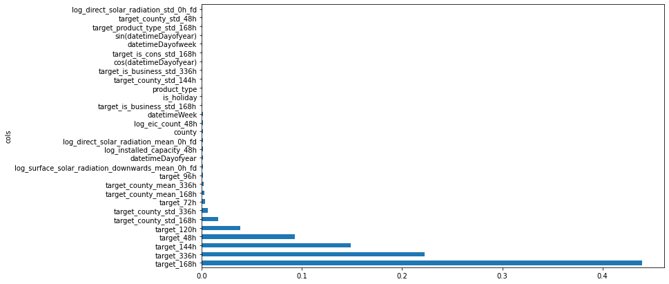
Figure 1: Plotting random forest feature importances
The targets’ 7-14 day history (particularly in relation to the county), forecasted sun exposure, installed capacity are most influential. The date and product type also appear among the top 30. In part 1, we discovered that the hardest examples were all consumption targets in Harjumaa, between 1-5pm on weekdays in Feb 2023. So far, the importances match intuition and prior observations.
Let’s zero-in on the most important features. With 358 columns, we’ll try keeping the top-scoring 30-40 features to keep things managable to study, which works out to a score of 0.0003 or more.
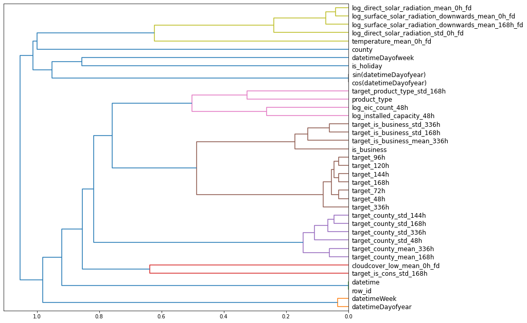
In the figure above, the most similar features are merged early, far from the tree’s root on the left.
The following appear closely related since they merged earliest:
datetime and row_id
cos(datetimeDayofyear) and sin(datetimeDayofyear)
Let’s see what we else can remove without losing accuracy. We’ll quickly train a small random forest and evaluate against OOB score; 1.0 for a perfect model and 0.0 for a random model.
We can near match our initial performance with just 35 features.
3 Partial dependence analysis
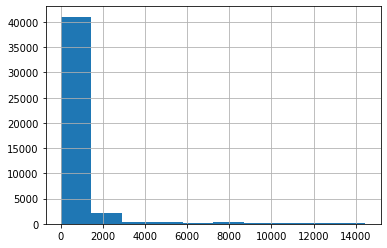
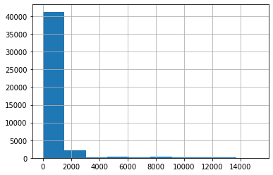
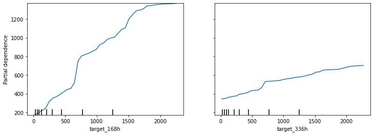
We saw that the top two predictors were target_168h and target_336h. To see how they vary with the target, we’ll first note where the bulk of the data falls:
Hide code
valid_xs_final['target_168h'].hist()
Hide code
valid_xs_final['target_168h'].describe()
count 44904.000000
mean 645.946106
std 1511.926025
min 0.000000
25% 75.920498
50% 208.003502
75% 599.245728
max 14455.158203
Name: target_168h, dtype: float64
Hide code
valid_xs_final['target_336h'].hist()
Hide code
valid_xs_final['target_336h'].describe()
count 44904.000000
mean 648.020203
std 1518.707153
min 0.000000
25% 76.580250
50% 213.181000
75% 601.848007
max 15213.572266
Name: target_336h, dtype: float64
In both cases, most of the values are between 0 and 600.
Figure 3: Partial dependence plots of the 2 strongest predictors
Over most of the observations, the model is more responsive to the 7-day lag (left) than to the 14-day lag (right). The jump in lag‑7 around 625 suggests a threshold where it has greater influence on the prediction, up to twice that of lag‑14. The jump around 1500 may be unreliable since the data there is sparse.
4 Out-of-Domain analysis
Next, we’ll try to improve by alleviating domain shift. To find features with high domain shift, we’ll re-label the data such that the model learns to predict whether a row belongs to the training or validation set and then look at its feature importances:
CPU times: user 4 µs, sys: 0 ns, total: 4 µs
Wall time: 9.3 µs
cols
imp
31
datetime
0.825639
12
datetimeDayofyear
0.066974
25
sin(datetimeDayofyear)
0.051183
17
datetimeWeek
0.018788
22
target_is_business_std_336h
0.014452
18
target_is_business_std_168h
0.006258
30
target_is_business_mean_336h
0.004764
34
temperature_mean_0h_fd
0.004439
23
target_is_cons_std_168h
0.003322
32
is_business
0.001758
datetime shifts the most since it is incremented most frequently. datetimeDayofyear, sin(datetimeDayofyear) and datetimeWeek increment less frequently and within a narrower range of values, so it makes sense why they shift less.
Let’s see if removing them helps, one at a time:
Hide code
%%timem = rf(xs_final, y)print('baseline', m_mae(m, valid_xs_final, valid_y))for c in ('datetime', 'datetimeDayofyear', 'sin(datetimeDayofyear)', 'datetimeWeek', 'target_is_business_std_336h'): m = rf(xs_final.drop(c,axis=1), y)print(c, m_mae(m, valid_xs_final.drop(c,axis=1), valid_y))
Our initial model, using 358 features and the whole dataset, achieved a 58.477 validation error. Our simplified model uses 32 features and 22% fewer records yet improves to a 53.214 validation error.
5 Modeling with a neural network
Show code
from numpy import randomrandom.seed(42)is_partial =Falseeval_month ='feb23'procs = [Categorify, Normalize]max_card =9000dep_var ='target'# need ['datetime', 'row_id'] for the splits, which are not in the final feature set. Dropped afterward. to_nn, final_splits = setup_training(is_partial, features_df[list(xs_final_time.columns) + ['datetime', 'row_id', dep_var]], pid_lookup_df, eval_month, procs, max_card)
n_pids_dropped from train: 4
pids_dropped from train: [14, 60, 20, 23]
Let’s confirm that TabularPandas correctly identified continuous and categorical variables:
Let’s see if we can improve still using the network’s categorical embeddings in a random forest.
Show code
def embed_features(learner, xs):# deep copy (creates new object w/ a copy of indices and data of original) xs = xs.copy()for i, feature inenumerate(learn.dls.cat_names):# get the embedding (move it to CPU first)# .cpu() see nn.ModuleList.cpu?# for learn.model.embeds, see learn.model?? emb = learn.model.embeds[i].cpu()# embed the categorical feature and return a df using the indices of xs# for embedding_dim see nn.Embedding??# join previously failed b/c col names overlap for each embedding feature# they were previously all to be named feature_0, feature_1, etc. new_feat = pd.DataFrame(emb(tensor(xs[feature], dtype=torch.int64)), index=xs.index, columns=[f"{feature}_{j}"for j inrange(emb.embedding_dim)])# drop the categorical feature xs.drop(columns=feature, inplace=True)# left join the embedded features w/ xs# returns nn's cat embeddings concatenated w/ original cont variables# the cont variables will be the same for the rf and the nn xs = xs.join(new_feat)return xs
%%timem_cat_emb = rf(embedded_xs, y)# pass m_cat_emb for the model. includes both cont variables and nn's cat embeddings# pass the embedded xs for both train and valid errorsprint("train mae: ", m_mae(m_cat_emb, embedded_xs, y))print("valid mae: ", m_mae(m_cat_emb, embedded_valid_xs, valid_y))print("OOB mae: ", mae(m_cat_emb.oob_prediction_, y))