Enefit - Predict Energy Behavior of Prosumers, part 3

1 Intro

In part 2, we modeled consumption behavior. In part 3, we’ll dig into production.

We’ll fetch the data and generate features:

%%time
d = Storage()
feature_generator = FeatureGenerator(d)

CPU times: user 20.8 s, sys: 4.16 s, total: 25 s
Wall time: 25.3 s

%%time 
features_df = feature_generator.generate_features()

CPU times: user 2min 32s, sys: 56.4 s, total: 3min 29s
Wall time: 3min 29s

features_df.shape

(2017824, 359)

And ensure we’re only looking at production from here on:

is_consumption_toggle = 0
features_df = features_df.loc[features_df["is_consumption"] == is_consumption_toggle]

print(features_df.loc[features_df["is_consumption"] == 0].shape, 
      features_df.loc[features_df["is_consumption"] == 1].shape)

(1008912, 359) (0, 359)

We’ll split the data:

from numpy import random
random.seed(42)

URLs.LOCAL_PATH = Path('/notebooks/kaggle/enefit')
save_path = URLs.LOCAL_PATH/'predict-energy-behavior-of-prosumers/pkl_files'
pid_lookup_df = load_pickle(save_path/'pid_lookup.pkl')

# includes dates of revealed_targets (2 days behind first eval day feb 1, 2023)
train_dates = {
    'part': [pd.to_datetime('2022-11-01 00:00:00'), pd.to_datetime('2023-01-29 23:00:00')],
    'full': [pd.to_datetime('2021-09-01 00:00:00'), pd.to_datetime('2023-01-29 23:00:00')]
}

eval_dates = {'feb23': [pd.to_datetime('2023-02-01 00:00:00'), pd.to_datetime('2023-02-28 23:00:00')],
              'mar23': [pd.to_datetime('2023-03-01 00:00:00'), pd.to_datetime('2023-03-31 23:00:00')],
              'apr23': [pd.to_datetime('2023-04-01 00:00:00'), pd.to_datetime('2023-04-30 23:00:00')],
              'may23': [pd.to_datetime('2023-05-01 00:00:00'), pd.to_datetime('2023-05-31 23:00:00')]
             }

def get_endpoints(is_partial, features_df, eval_month:str):

    if is_partial:
        train_dates_conds = [features_df['datetime'] == train_dates['part'][0], 
                             features_df['datetime'] == train_dates['part'][1]
                            ]
    else:
        train_dates_conds = [features_df['datetime'] == train_dates['full'][0], 
                             features_df['datetime'] == train_dates['full'][1]
                            ]
    
    train_endpoints = [features_df['datetime'][train_dates_conds[0]].index[0], 
                       features_df['datetime'][train_dates_conds[1]].index[-1]
                      ]

    valid_dates_cond = [features_df['datetime'] == eval_dates[eval_month][0], 
                        features_df['datetime'] == eval_dates[eval_month][1]
                       ]

    valid_endpoints = [features_df['datetime'][valid_dates_cond[0]].index[0], 
                       features_df['datetime'][valid_dates_cond[1]].index[-1]
                      ]

    return train_endpoints, valid_endpoints

def get_splits(is_partial, features_df, eval_month:str):
    train_endpoints, valid_endpoints = get_endpoints(is_partial, features_df, eval_month)
    train = features_df.iloc[train_endpoints[0]:train_endpoints[1]+1].index.tolist()
    valid = features_df.iloc[valid_endpoints[0]:valid_endpoints[1]+1].index.tolist()
    splits = (train, valid)
    return splits

def drop_pids_from_train(features_df, splits, pid_lookup_df):
    
    max_n_pids_to_drop = 7
    training_pids = set(features_df.iloc[splits[0]].merge(pid_lookup_df, how='left', on=['row_id'])['prediction_unit_id'].unique().tolist())
    valid_pids = set(features_df.iloc[splits[1]].merge(pid_lookup_df, how='left', on=['row_id'])['prediction_unit_id'].unique().tolist())
    intersection_pids = list(training_pids.intersection(valid_pids))
    
    # pids drop list may not be continuous or sorted.
    intersection_pids.sort() 

    # drop from those not already missing in the valid fold, THIS ROUND.
    # to get the number of pids to drop THIS ROUND, pick a random int b/w 1 and the max allowed to drop.
    n_pids_drop = random.randint(1, max_n_pids_to_drop) 

    # to get the pids to drop, index intersection_pids w/ a random int b/w 0 and its last index. repeat for the n_pids_drop chosen for THIS ROUND. 
    pids_to_drop = [random.randint(0, len(intersection_pids)-1) for i in range(n_pids_drop)]

    # drop only from train (slice features_df by training dates from the endpoints, join to lookup pids, mask, apply the mask to the slice)
    # get its indices
    mask = features_df.iloc[splits[0]].merge(pid_lookup_df, how='left', on=['row_id'])['prediction_unit_id'].isin(pids_to_drop)

    return mask, n_pids_drop, pids_to_drop

def setup_tabular_pandas(features_df, procs, max_card, splits, dep_var='target'):  
    # variables
    cont, cat = cont_cat_split(features_df, max_card, dep_var=dep_var)

    # setup object
    return TabularPandas(features_df, procs, cat, cont, y_names=dep_var, splits=splits)

def setup_training(is_partial, features_df, pid_lookup_df, eval_month, procs, max_card):

    features_df = features_df.reset_index(drop=True)      
    tmp_splits = get_splits(is_partial, features_df, eval_month)

    # _get_splits -> _get_pids_drop_mask needs row_id to join pid_lookup_df
    pid_mask, n_pids_dropped, pids_dropped = drop_pids_from_train(features_df, tmp_splits, pid_lookup_df)
    valid_buffer = pd.Series(np.zeros(len(tmp_splits[1]), dtype='bool'))
    pid_mask = pd.concat([pid_mask, valid_buffer])
    pid_mask.index = tmp_splits[0] + tmp_splits[1]
    tmp_df = features_df.iloc[tmp_splits[0]+tmp_splits[1]][~pid_mask]
    features_df_final = tmp_df.reset_index(drop=True)

    # re-compute the splits after applying pid_mask.
    final_splits = get_splits(is_partial, features_df_final, eval_month)
    del tmp_splits, tmp_df
    gc.collect()

    # setup training
    procs = procs
    max_card = max_card
    to = setup_tabular_pandas(features_df_final, procs, max_card, final_splits)

    print(f"n_pids_dropped from train: {n_pids_dropped}")
    print(f"pids_dropped from train: {pids_dropped}")
    
    return to, final_splits

is_partial = False
eval_month = 'feb23'
procs = [Categorify]
max_card = 20

to, final_splits = setup_training(is_partial, features_df, pid_lookup_df, eval_month, procs, max_card)

n_pids_dropped from train: 4
pids_dropped from train: [14, 60, 20, 23]

def get_train_and_valid(to):
    xs, y = to.train.xs, to.train.y
    valid_xs, valid_y = to.valid.xs, to.valid.y
    
    return xs, y, valid_xs, valid_y

xs, y, valid_xs, valid_y = get_train_and_valid(to)
print(len(xs), len(y), len(valid_xs), len(valid_y))

765510 765510 44904 44904

2 Modeling with trees

Now we’re in business. Let’s train a random forest and look at its feature importances:

def mae(preds, y): return round((preds-y).abs().mean(), 6)
def m_mae(m, xs, y): return mae(m.predict(xs), y)

def rf(xs, y, n_estimators=40, max_features=0.5, min_samples_leaf=5, **kwargs):
    return RandomForestRegressor(n_jobs=-1, 
                                 n_estimators=n_estimators,
                                 max_samples=int(0.5*len(xs)), 
                                 max_features=max_features,
                                 min_samples_leaf=min_samples_leaf, 
                                 oob_score=True).fit(xs, y)

%%time
m = rf(xs, y)

CPU times: user 2h 56min 33s, sys: 26.2 s, total: 2h 57min
Wall time: 30min 56s

print("train mae: ", m_mae(m, xs, y))
print("valid mae: ", m_mae(m, valid_xs, valid_y))
print("OOB error: ", mae(m.oob_prediction_, y))

train mae:  11.673442
valid mae:  49.841143
OOB error:  16.204788

def rf_feat_importance(m, df):
    return pd.DataFrame({'cols':df.columns, 'imp':m.feature_importances_}
                       ).sort_values('imp', ascending=False)

def plot_fi(fi):
    return fi.plot('cols', 'imp', 'barh', figsize=(12,7), legend=False)

fi = rf_feat_importance(m, xs)
fi[:10]

	cols	imp
286	target_48h	0.307471
291	target_168h	0.175694
292	target_336h	0.108706
290	target_144h	0.083727
27	log_direct_solar_radiation_mean_0h_fd	0.047537
28	log_surface_solar_radiation_downwards_mean_0h_fd	0.043826
289	target_120h	0.031447
18	log_installed_capacity_48h	0.019918
287	target_72h	0.019280
288	target_96h	0.014335

plot_fi(fi[:30]);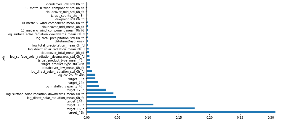

Figure 1: Plotting random forest feature importances

The targets’ 7-14 day history, installed capacity, and the forecasted weather are the most influential features. We’ll focus on the top-scoring 40.

fi[:40]

	cols	imp
286	target_48h	0.307471
291	target_168h	0.175694
292	target_336h	0.108706
290	target_144h	0.083727
27	log_direct_solar_radiation_mean_0h_fd	0.047537
...	...	...
42	log_total_precipitation_mean_168h_fd	0.001138
20	dewpoint_mean_0h_fd	0.001080
312	target_county_mean_168h	0.001049
50	10_metre_v_wind_component_std_0h_fd	0.001026
37	10_metre_u_wind_component_mean_168h_fd	0.001025

40 rows × 2 columns

to_keep = fi[fi.imp>0.001].cols
len(xs.columns), len(to_keep)

(358, 41)

xs_imp = xs[to_keep]
valid_xs_imp = valid_xs[to_keep]

%%time
m = rf(xs_imp, y)

CPU times: user 19min 45s, sys: 2.81 s, total: 19min 48s
Wall time: 3min 32s

print("train mae: ", m_mae(m, xs_imp, y))
print("valid mae: ", m_mae(m, valid_xs_imp, valid_y))
print("OOB error: ", mae(m.oob_prediction_, y))

train mae:  12.529778
valid mae:  14.233786
OOB error:  16.768616

We’ve achieved a dramatic improvement without much change in both the training and OOB errors. We’ll remove redundancy next.

cluster_columns(xs_imp, figsize=(12, 11))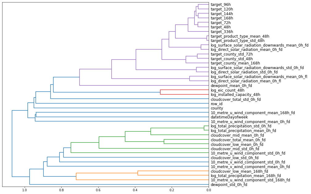

Figure 2: Visualizing feature similarity

In the figure above, the most similar features are merged early, far from the tree’s root on the left. There don’t appear to be potentially redundant features, so we’ll proceed.

xs_final = xs_imp
valid_xs_final = valid_xs_imp

3 Partial dependence analysis

We saw that the top two predictors were target_48h and target_168h. To see how they vary with the target, we’ll first note where the bulk of the data falls:

valid_xs_final['target_48h'].hist()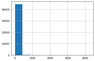

valid_xs_final['target_48h'].describe()

count    44904.000000
mean        15.214073
std         89.586014
min          0.000000
25%          0.000000
50%          0.052000
75%          2.450000
max       4253.659180
Name: target_48h, dtype: float64

valid_xs_final['target_168h'].hist()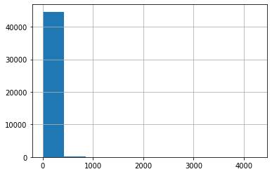

valid_xs_final['target_168h'].describe()

count    44904.000000
mean        14.775428
std         89.288246
min          0.000000
25%          0.000000
50%          0.040000
75%          2.234250
max       4253.659180
Name: target_168h, dtype: float64

print(len(valid_xs_final['target_48h'][valid_xs_final['target_48h'] > 100]), 
           len(valid_xs_final['target_168h'][valid_xs_final['target_168h'] > 100]))

1392 1336

In both cases, most of the values are between 0 and 3.

from sklearn.inspection import partial_dependence
from sklearn.inspection import PartialDependenceDisplay

fig,ax = plt.subplots(figsize=(12, 4))
PartialDependenceDisplay.from_estimator(m, valid_xs_final, ['target_48h', 'target_168h'], 
                                        grid_resolution=40, ax=ax)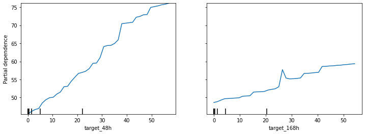

Figure 3: Partial dependence plots of the 2 strongest predictors

Over most of the observations, the model is ~5x more responsive to the 2-day lag (left) than to the 7-day lag (right). The jumps in lag-2 and lag-7 beyond the 0-3 range are likely unreliable due to data sparsity.

4 Out-of-Domain analysis

Next we’ll alleviate domain shift. Let’s find the features that exhibit the most shift:

%time
df_dom = pd.concat([xs_final, valid_xs_final])
is_valid = np.array([0]*len(xs_final) + [1]*len(valid_xs_final))

m_dom = rf(df_dom, is_valid)
rf_feat_importance(m_dom, df_dom)[:10]

CPU times: user 4 µs, sys: 0 ns, total: 4 µs
Wall time: 10 µs

	cols	imp
32	row_id	0.955003
36	dewpoint_mean_0h_fd	0.018782
40	cloudcover_low_mean_168h_fd	0.006110
24	10_metre_v_wind_component_mean_0h_fd	0.003335
39	10_metre_u_wind_component_mean_168h_fd	0.002816
12	cloudcover_low_mean_0h_fd	0.002591
33	10_metre_u_wind_component_std_168h_fd	0.002023
28	10_metre_u_wind_component_std_0h_fd	0.002015
35	log_total_precipitation_mean_168h_fd	0.001318
16	cloudcover_total_mean_0h_fd	0.001216

It makes sense thatrow_id shifts the most since it is incremented most frequently. Intuitively, it shouldn’t bear any inherent influence on the target although it has shown up among the top 40 most influential features. It could be one of the features driving some of the overfitting. Let’s try removing it.

%%time
m = rf(xs_final, y)
print('baseline', m_mae(m, valid_xs_final, valid_y))

c = 'row_id'
m = rf(xs_final.drop(c,axis=1), y)
print(c, m_mae(m, valid_xs_final.drop(c,axis=1), valid_y))

baseline 14.881774
row_id 13.242199
CPU times: user 37min 18s, sys: 4.24 s, total: 37min 22s
Wall time: 6min 44s

time_vars = ['row_id']
xs_final_time = xs_final.drop(time_vars, axis=1)
valid_xs_time = valid_xs_final.drop(time_vars, axis=1)

print("train mae: ", m_mae(m, xs_final_time, y))
print("OOB error: ", mae(m.oob_prediction_, y))

train mae:  12.647144
OOB error:  16.883626

Looks good. Let’s try dropping data prior to Jan 2022:

filt = xs['datetimeYear']>1
xs_filt = xs_final_time[filt]
y_filt = y[filt]

%%time
m = rf(xs_filt, y_filt)
print("train mae: ", m_mae(m, xs_filt, y_filt))
print("valid mae: ", m_mae(m, valid_xs_time, valid_y))
print("OOB error: ", mae(m.oob_prediction_, y_filt))

train mae:  13.872813
valid mae:  13.078788
OOB error:  18.6608
CPU times: user 14min 13s, sys: 1.93 s, total: 14min 15s
Wall time: 2min 35s

len(xs.columns), len(xs_filt.columns)

(358, 40)

len(xs), len(xs_filt)

(765510, 594257)

The forest has a slightly higher training error than validation error, which points to good generalization. But the OOB error exceeds the forests’ validation error, which shows that the individual trees are overfitting their training subsets. This may be because this forest includes only 40 trees, so the OOB error may be unstable. Using more trees may alleviate the discrepancy. For now, we’ll keep going with a neural network.

5 Modeling with a neural network

from numpy import random
random.seed(42)

is_partial = False
eval_month = 'feb23'
procs = [Categorify, Normalize]
max_card = 9000
dep_var = 'target'

# need ['datetime', 'row_id'] for the splits, which are not in the final feature set. Dropped afterward. 
to_nn, final_splits = setup_training(is_partial, 
                                     features_df[list(xs_final_time.columns) + ['datetime', 'row_id', dep_var]], 
                                     pid_lookup_df, 
                                     eval_month, 
                                     procs, 
                                     max_card)

n_pids_dropped from train: 4
pids_dropped from train: [14, 60, 20, 23]

Let’s confirm that TabularPandas correctly identified continuous and categorical variables:

to_nn.cont_names.remove('row_id')
to_nn.cat_names.remove('datetime')

{'cont_names': list(to_nn.cont_names), 
 'cat_names': list(to_nn.cat_names)
}

{'cont_names': ['target_48h',
  'target_168h',
  'target_336h',
  'target_144h',
  'log_direct_solar_radiation_mean_0h_fd',
  'log_surface_solar_radiation_downwards_mean_0h_fd',
  'target_120h',
  'log_installed_capacity_48h',
  'target_72h',
  'target_96h',
  'log_eic_count_48h',
  'log_direct_solar_radiation_std_0h_fd',
  'cloudcover_low_mean_0h_fd',
  'target_product_type_std_48h',
  'target_product_type_mean_48h',
  'log_surface_solar_radiation_downwards_std_0h_fd',
  'cloudcover_total_mean_0h_fd',
  'log_direct_solar_radiation_mean_0h_fl',
  'log_total_precipitation_mean_0h_fd',
  'log_total_precipitation_std_0h_fd',
  'log_surface_solar_radiation_downwards_mean_0h_fl',
  '10_metre_u_wind_component_mean_0h_fd',
  'cloudcover_mid_mean_0h_fd',
  '10_metre_v_wind_component_mean_0h_fd',
  'dewpoint_std_0h_fd',
  'target_county_std_48h',
  'cloudcover_mid_std_0h_fd',
  '10_metre_u_wind_component_std_0h_fd',
  'cloudcover_low_std_0h_fd',
  'target_county_std_72h',
  '10_metre_u_wind_component_std_168h_fd',
  'cloudcover_total_std_0h_fd',
  'log_total_precipitation_mean_168h_fd',
  'dewpoint_mean_0h_fd',
  'target_county_mean_168h',
  '10_metre_v_wind_component_std_0h_fd',
  '10_metre_u_wind_component_mean_168h_fd',
  'cloudcover_low_mean_168h_fd'],
 'cat_names': ['datetimeDayofweek', 'county']}

And train the network:

def nn_mae(preds, y): return torch.round((preds - y).abs().mean(), decimals=6)

bs = 1024
dls = to_nn.dataloaders(bs)

y = to_nn.train.y
y.min(),y.max()

(0.0, 7814.313)

y_max_factor = 3
np.ceil(y_max_factor*y.max())

23443.0

y_max = np.ceil(y_max_factor*y.max())
layers = [1000, 500]

learn = tabular_learner(dls, y_range=(0, y_max), layers=layers,
                        n_out=1, loss_func=F.l1_loss)

learn.lr_find(suggest_funcs=[slide, valley])

SuggestedLRs(slide=6.309573450380412e-07, valley=0.0012022644514217973)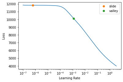

We’ll use a 1e-3 learning rate and train for a few epochs:

learn.fit_one_cycle(5, 1e-3)

epoch	train_loss	valid_loss	time
0	385.152618	89.120911	00:18
1	28.974539	13.420791	00:16
2	23.203011	13.486762	00:15
3	18.423313	11.819149	00:19
4	17.882912	11.734632	00:19

And view the predictions (scroll to the right end):

learn.show_results()

	county	datetimeWeek	is_holiday	product_type	datetimeDayofweek	is_business	target_168h	target_336h	target_144h	target_48h	target_120h	target_county_std_168h	target_county_std_336h	target_72h	target_county_mean_168h	target_county_mean_336h	target_96h	log_surface_solar_radiation_downwards_mean_0h_fd	log_installed_capacity_48h	log_direct_solar_radiation_mean_0h_fd	log_eic_count_48h	target_is_business_std_168h	target_county_std_144h	target_is_cons_std_168h	sin(datetimeDayofyear)	target_product_type_std_168h	target_county_std_48h	log_direct_solar_radiation_std_0h_fd	log_surface_solar_radiation_downwards_mean_168h_fd	target_is_business_mean_336h	cloudcover_low_mean_0h_fd	temperature_mean_0h_fd	target	target_pred
0	15.0	8.0	1.0	2.0	6.0	2.0	-0.262886	-0.239930	-0.260615	-0.253527	-0.262182	-0.202138	-0.307286	-0.247566	-0.058346	-0.111946	-0.253991	-0.889688	-0.362890	-0.827848	-0.497701	0.772622	-0.282687	0.029818	1.397399	-0.679453	-0.069211	-0.751869	-0.883614	0.964591	1.459237	-1.211010	127.239998	134.697464
1	4.0	7.0	1.0	2.0	7.0	2.0	-0.330954	-0.323535	-0.334922	-0.338295	-0.335445	-0.187287	-0.164677	-0.336010	-0.142387	-0.084139	-0.337699	-0.889688	-0.912775	-0.827848	-0.941712	0.653363	-0.223687	-0.136800	1.306189	-0.697084	-0.247657	-0.751869	-0.883614	0.893931	0.495124	-0.811021	30.806000	46.891251
2	5.0	5.0	1.0	2.0	4.0	1.0	-0.344467	-0.342138	-0.347831	-0.347422	-0.344598	-0.340768	-0.363358	-0.347488	-0.202386	-0.229166	-0.345382	-0.889688	-0.594519	-0.827848	-0.497701	-0.594282	-0.368845	0.176550	0.988584	-0.697989	-0.412845	-0.751869	-0.883614	-0.523382	1.371129	-0.838103	19.188999	25.702089
3	3.0	7.0	1.0	2.0	7.0	2.0	-0.289490	-0.279803	-0.255431	-0.248302	-0.272753	-0.446600	-0.421871	-0.239236	-0.453071	-0.407710	-0.268927	1.030597	-1.226184	0.143757	-1.027643	1.120253	-0.424511	0.571177	1.306189	-0.669880	-0.322436	2.449245	1.079126	0.928739	1.283659	-0.868476	96.105003	73.928062
4	16.0	8.0	1.0	2.0	7.0	2.0	-0.183543	-0.193427	-0.194822	-0.215773	-0.188846	-0.686955	-0.673423	-0.192416	-0.496016	-0.502450	-0.170561	-0.889688	0.245607	-0.827848	-0.201525	0.982311	-0.657861	0.407525	1.411405	-0.635931	-0.685927	-0.751869	-0.883614	0.968042	-0.691459	-1.517333	188.632004	208.133240
5	4.0	7.0	1.0	2.0	4.0	2.0	-0.330865	-0.320998	-0.334936	-0.338640	-0.330539	-0.167406	-0.119311	-0.336651	-0.143195	-0.080749	-0.332357	-0.889688	-0.912775	-0.827848	-0.941712	1.373603	-0.117017	1.038111	1.256177	-0.603400	-0.202103	-0.751869	-0.883614	1.533619	1.582296	-0.634451	46.298000	53.170086
6	4.0	5.0	1.0	4.0	4.0	2.0	0.575863	0.502346	0.570968	0.550353	0.558134	-0.204478	-0.250005	0.511721	-0.218346	-0.252642	0.532916	-0.889688	1.269762	-0.827848	0.525585	0.855744	-0.211454	0.152174	0.988584	1.158699	-0.226203	-0.751869	-0.883614	0.865195	1.446751	-0.840503	1089.301025	1143.673706
7	11.0	6.0	1.0	2.0	6.0	1.0	-0.285181	-0.302084	-0.304559	-0.306237	-0.307852	-0.487169	-0.495147	-0.307560	-0.255986	-0.339585	-0.306730	-0.889688	-0.087960	-0.827848	0.423409	-0.373181	-0.508577	0.262175	1.166752	-0.644339	-0.466170	-0.751869	-0.883614	-0.397293	-1.234372	-1.086801	70.140999	70.644394
8	16.0	6.0	1.0	2.0	7.0	1.0	-0.296332	-0.299581	-0.313292	-0.314098	-0.311906	-0.637992	-0.634026	-0.332257	-0.458398	-0.461850	-0.308999	0.983235	-0.584762	0.296804	0.348233	-0.691865	-0.314547	0.217005	1.185220	-0.742475	-0.406558	2.658769	1.114219	-0.522843	-0.189756	-0.665068	61.251999	75.555504

These look reasonable. Let’s train a few more epochs:

learn = tabular_learner(dls, y_range=(0, y_max), layers=layers,
                        n_out=1, loss_func=F.l1_loss)

learn.fit_one_cycle(10, 1e-3)

epoch	train_loss	valid_loss	time
0	1058.503296	307.893738	00:18
1	33.334896	16.926445	00:17
2	26.946150	12.923368	00:16
3	21.992962	12.006287	00:15
4	20.392881	12.321980	00:16
5	19.228310	11.995186	00:17
6	17.760178	11.779169	00:15
7	16.319954	11.705316	00:15
8	15.099010	11.637057	00:15
9	14.862897	11.599226	00:16

preds, targs = learn.get_preds()
print("nn valid mae: ", nn_mae(preds, targs))

nn valid mae:  tensor(11.5992)

We again see a higher training error than validation error. This may be attributable to regularization, where training is made harder to prevent overfitting. fastai’s tabular_learner uses Dropout, weight decay, and batch normalization by default. It’s also possible that the validation set used during our development process is simply easier than the training set. In part 4, we will perform cross-validation, where we’ll train and evaluate on 3 different data splits, which will give us a better idea of our performance.

Let’s see whether ensembling can take us further.

6 Ensembling

rf_preds = m.predict(valid_xs_time)
ens_preds = (to_np(preds.squeeze()) + rf_preds) /2

(ens_preds - valid_y).abs().mean()

11.833211038886864

7 Entity embeddings in a random forest

Let’s try using the network’s categorical embeddings in a random forest.

def embed_features(learner, xs):
    # deep copy (creates new object w/ a copy of indices and data of original)
    xs = xs.copy()
    for i, feature in enumerate(learn.dls.cat_names):
        
        # get the embedding (move it to CPU first)
        # .cpu() see nn.ModuleList.cpu?
        # for learn.model.embeds, see learn.model??
        emb = learn.model.embeds[i].cpu()
        
        # embed the categorical feature and return a df using the indices of xs
        # for embedding_dim see nn.Embedding??
        # join previously failed b/c col names overlap for each embedding feature
        # they were previously all to be named feature_0, feature_1, etc.
        new_feat = pd.DataFrame(emb(tensor(xs[feature], dtype=torch.int64)), 
                                index=xs.index, 
                                columns=[f"{feature}_{j}" for j in range(emb.embedding_dim)])
        
        # drop the categorical feature
        xs.drop(columns=feature, inplace=True)
        
        # left join the embedded features w/ xs
        # returns nn's cat embeddings concatenated w/ original cont variables
        # the cont variables will be the same for the rf and the nn
        xs = xs.join(new_feat)
    return xs

embedded_xs = embed_features(learn, learn.dls.train.xs)
embedded_valid_xs = embed_features(learn, learn.dls.valid.xs)
embedded_xs.shape, embedded_valid_xs.shape

((765510, 51), (44904, 51))

embedded_xs.columns

Index(['target_48h', 'target_168h', 'target_336h', 'target_144h',
       'log_direct_solar_radiation_mean_0h_fd',
       'log_surface_solar_radiation_downwards_mean_0h_fd', 'target_120h',
       'log_installed_capacity_48h', 'target_72h', 'target_96h',
       'log_eic_count_48h', 'log_direct_solar_radiation_std_0h_fd',
       'cloudcover_low_mean_0h_fd', 'target_product_type_std_48h',
       'target_product_type_mean_48h',
       'log_surface_solar_radiation_downwards_std_0h_fd',
       'cloudcover_total_mean_0h_fd', 'log_direct_solar_radiation_mean_0h_fl',
       'log_total_precipitation_mean_0h_fd',
       'log_total_precipitation_std_0h_fd',
       'log_surface_solar_radiation_downwards_mean_0h_fl',
       '10_metre_u_wind_component_mean_0h_fd', 'cloudcover_mid_mean_0h_fd',
       '10_metre_v_wind_component_mean_0h_fd', 'dewpoint_std_0h_fd',
       'target_county_std_48h', 'cloudcover_mid_std_0h_fd',
       '10_metre_u_wind_component_std_0h_fd', 'cloudcover_low_std_0h_fd',
       'target_county_std_72h', '10_metre_u_wind_component_std_168h_fd',
       'cloudcover_total_std_0h_fd', 'log_total_precipitation_mean_168h_fd',
       'dewpoint_mean_0h_fd', 'target_county_mean_168h',
       '10_metre_v_wind_component_std_0h_fd',
       '10_metre_u_wind_component_mean_168h_fd', 'cloudcover_low_mean_168h_fd',
       'datetimeDayofweek_0', 'datetimeDayofweek_1', 'datetimeDayofweek_2',
       'datetimeDayofweek_3', 'datetimeDayofweek_4', 'county_0', 'county_1',
       'county_2', 'county_3', 'county_4', 'county_5', 'county_6', 'county_7'],
      dtype='object')

%%time
m_cat_emb = rf(embedded_xs, y)
# pass m_cat_emb for the model. includes both cont variables and nn's cat embeddings
# pass the embedded xs for both train and valid errors
print("train mae: ", m_mae(m_cat_emb, embedded_xs, y))
print("valid mae: ", m_mae(m_cat_emb, embedded_valid_xs, valid_y))
print("OOB mae: ", mae(m_cat_emb.oob_prediction_, y))

train mae:  12.522175
valid mae:  13.452001
OOB mae:  16.744852
CPU times: user 21min 59s, sys: 3.78 s, total: 22min 3s
Wall time: 3min 59s

8 Next steps

The neural network gave us the best MAE (11.59). However, since the random forest and neural network ensemble scores a close 11.83 while mitigating each model’s weaknesses, we will proceed with the ensemble.

In part 4, we will finally see whether modeling consumption and production independently will give more accurate overall predictions than a modeling them together.